Home  · Charts  · Time Control

Trace Agent

Tools
pmdatrace
pmtrace
pminfo

This chapter of the Performance Co-Pilot tutorial discusses application instrumentation using the trace PMDA (Performance Metrics Domain Agent). The trace agent has similar aims to the Memory Mapped Values (MMV) agent, in that both provide interfaces for application instrumentation. The main differences are:

• The trace PMDA is a predecessor to MMV, and it is expected that most instrumented applications would use MMV.
• The trace interface uses sockets for communication between applications and agent, MMV uses memory mapped files.  This is heavier weight but allows for instrumentation to be sent between hosts, optionally.
• MMV allows the application to completely specify every aspect of each metric it exports, the trace agent has a small number of metrics with relatively fixed metadata, and each applications instrumentation is exported as an instance of these fixed metrics.
• This fixed nature of the trace metrics caters for existance of the program pmtrace allowing simple instrumentation from the shell.

For an explanation of Performance Co-Pilot terms and acronyms, consult the PCP glossary.

• Overview
• Trace Agent Design
  • Application Interaction
  • Sampling Techniques
  • Configuring the Trace Agent
• The Trace API
  • Transactions
  • Point Tracing
  • Observations/Counters
  • Configuring the Trace library
• Instrumenting Applications to Export Performance Data

This document provides an introduction to the design of the trace agent, in an effort to explain how to configure the agent optimally for a particular problem domain.  This will be most useful as a supplement to the functional coverage which the manual pages provide to both the agent and the library interfaces.

Details of the use of the trace agent, and the associated library (libpcp_trace) for instrumenting applications, are also discussed.

In a command shell enter: # . /etc/pcp.conf # cd $PCP_PMDAS_DIR/trace # ./Install Export a value, from the shell using: $ pmtrace -v 100 "database-users" $ pminfo -f trace

Application Interaction

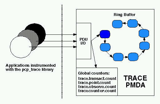
The diagram below describes the general state maintained within the trace agent.  Applications which are linked with the libpcp_trace library make calls through the trace Applications Programmer Interface (API), resulting in inter-process communication of trace data between the application and the trace agent.  This data consists of an identification tag, and the performance data associated with that particular tag.  The trace agent aggregates the incoming information and periodically updates the exported summary information to describe activity in the recent past.

As each PDU (Protocol Data Unit) is received, its data is stored in the current working buffer, and at the same time the global counter associated with the particular tag contained within the PDU is incremented.  The working buffer contains all performance data which has arrived since the previous time interval elapsed, and is discussed in greater detail in the Rolling Window Sampling Technique section below.

Sampling Techniques

The trace agent employs a rolling window periodic sampling technique.  The recency of the data exported by the agent is determined by its arrival time at the agent in conjunction with the length of the sampling period being maintained by the trace agent.  Through the use of rolling window sampling, the trace agent is able to present a more accurate representation of the available trace data at any given time.

The metrics affected by the agents rolling window sampling technique are:

• trace.transact.rate
• trace.transact.ave_time
• trace.transact.min_time
• trace.transact.max_time
• trace.point.rate
• trace.observe.rate
• trace.counter.rate

The remaining metrics are either global counters, control metrics, or the last seen observation/counter value.  All metrics exported by the trace agent are explained in detail in the API section below.

Simple periodic sampling

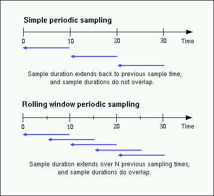
This technique uses a single historical buffer to store the history of events which have occurred over the sampling interval.  As events occur they are recorded in the working buffer.  At the end of each sampling interval the working buffer (which at that time holds the historical data for the sampling interval just finished) is copied into the historical buffer, and the working buffer is cleared (ready to hold new events from the sampling interval now starting).

Rolling window periodic sampling

In contrast to simple periodic sampling with its single historical buffer, the rolling window periodic sampling technique maintains a number of separate buffers.  One buffer is marked as the current working buffer, and the remainder of the buffers hold historical data.  As each event occurs, the current working buffer is updated to reflect this.

At a specified interval (which is a function of the number of historical buffers maintained) the current working buffer and the accumulated data which it holds is moved into the set of historical buffers, and a new working buffer is used.

The primary advantage of the rolling window approach is that at the point where data is actually exported, the data which is exported has a higher probability of reflecting a more recent sampling period than the data exported using simple periodic sampling.

The data collected over each sample duration and exported using the rolling window technique provides a more up-to-date representation of the activity during the most recently completed sample duration.

The trace agent allows the length of the sample duration to be configured, as well as the number of historical buffers which are to be maintained.  The rolling window is implemented in the trace agent as a ring buffer (as shown earlier in the "Trace agent Overview" diagram), such that when the current working buffer is moved into the set of historical buffers, the least recent historical buffer is cleared of data and becomes the new working buffer.

Example of window periodic sampling

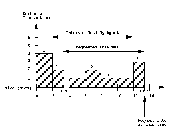
Consider the scenario where one wants to know the rate of transactions over the last 10 seconds.  To do this one would set the sampling rate for the trace agent to be 10 seconds and would fetch the metric trace.transact.rate. So if in the last 10 seconds we had 8 transactions take place then we would have a transaction rate of 8/10 or 0.8 transactions per second.

As mentioned above, the trace agent does not actually do this.  It instead does its calculations automatically at a subinterval of the sampling interval.  Consider the example above with a calculation subinterval of 2 seconds.  Please refer to the bar chart below.  At time 13.5 secs the user requests the transaction rate and is told it is has a value of 0.7 transactions per second.  In actual fact, the transaction rate was 0.8 but the agent has done its calculations on the sampling interval from 2 secs to 12 secs and not from 3.5 secs to 13.5 secs. Every 2 seconds it will do the metrics calculations on the last 10 seconds at that time.  It does this for efficiency and so it is not driven each time to do a calculation for a fetch request.

Configuring the Trace agent

The trace agent is configurable primarily through command line options.  The list of command line options presented below is not exhaustive, but covers those options which are particularly relevant to tuning the manner in which performance data is collected.

Options:

Access Controls

host-based access control is offered by the trace agent, allowing and disallowing connections from instrumented applications running on specified hosts or groups of hosts.  Limits to the number of connections allowed from individual hosts can also be mandated

Sample Duration

interval over which metrics are to be maintained before being discarded.

Number of Historical Buffers

the data maintained for the sample duration is held in a number of internal buffers within the trace agent.  This number is configurable, allowing the rolling window effect to be tuned (within the sample duration)

Observation/Counter Metric Units

since the data being exported by the trace.observe.value and trace.counter.value metrics is user-defined, the trace agent by default exports these metrics with a type of "none".  A framework is provided allowing this to be made more specific (bytes per second, for example), allowing the exported values to be plotted along with other performance metrics of similar units by tools like pmchart)

Instance Domain Refresh

the set of instances exported for each of the trace metrics can be cleared through the storable trace.control.reset metric.

The libpcp_trace Applications Programmer Interface (API) may be called from C, C++, Fortran, and Java.  Each language has access to the complete set of functionality offered by libpcp_trace, although in some cases the calling conventions differ slightly between languages.  An overview of each of the different tracing mechanisms offered by the API follows, as well as an explanation of their mappings to the actual performance metrics exported by the trace agent.

Transactions

Paired calls to the pmtracebegin(3) and pmtraceend(3) API functions will result in transaction data being sent to the agent with a measure of the time interval between the two calls (which is assumed to be the transaction service time).  Using the pmtraceabort(3) call causes data for that particular transaction to be discarded. Transaction data is exported through the trace agents trace.transact metrics.

trace.transact.count

running count for each transaction type seen since the trace agent started

trace.transact.rate

the average rate at which each transaction type is completed, calculated over the last sample duration

trace.transact.ave_time

the average service time per transaction type, calculated over the last sample duration

trace.transact.min_time

minimum service time per transaction type within the last sample duration

trace.transact.max_time

maximum service time per transaction type within the last sample duration

trace.transact.total_time

cumulative time spent processing each transaction since the trace agent started running

Point tracing

Point tracing allows the application programmer to export metrics related to salient events.  The pmtracepoint(3) function is most useful when start and end points are not well defined, eg. when the code branches in such a way that a transaction cannot be clearly identified, or when processing does not follow a transactional model, or the desired instrumentation is akin to event rates rather than event service times.  This data is exported through the trace.point metrics.

trace.point.count

running count of point observations for each tag seen since the trace agent started

trace.point.rate

the average rate at which observation points occur for each tag, within the last sample duration

Observations/Counters

The pmtraceobs(3) and pmtracecounter(3) functions have similar semantics to pmtracepoint(3), but also allow an arbitrary numeric value to be passed to the trace agent.  The most recent value for each tag is then immediately available from the agent. Observation and counter data is exported through the trace.observe and trace.counter metrics, and these differ only in the PMAPI semantics associated with their respective value metrics (the PMAPI semantics for these two metrics is "instantaneous" or "counter" - refer to the PMAPI(3) manual page for details on PMAPI metric semantics).

trace.observe.count, trace.counter.count

running count of observations/counters seen since the trace agent started

trace.observe.rate, trace.counter.rate

the average rate at which observations/counters for each tag occur, calculated over the last sample duration

trace.observe.value, trace.counter.value

the numeric value associated with the observation/counter last seen by the agent

Configuring the Trace library

The trace library is configurable through the use of environment variables, as well as through state flags, which provide diagnostic output and enable or disable the configurable functionality within the library.

Environment variables:

PCP_TRACE_HOST

the name of the host where the trace agent is running

PCP_TRACE_PORT

TCP/IP port number on which the trace agent is accepting client connections

PCP_TRACE_TIMEOUT

number to seconds to wait until assuming that the initial connection is not going to be made, and timeout is to occur (the default is three seconds)

PCP_TRACE_REQTIMEOUT

number of seconds to allow before timing out on awaiting acknowledgement from the trace agent after trace data has been sent to it.  This variable has no effect in the asynchronous trace protocol (refer to PMTRACE_STATE_ASYNC under `State Flags', below)

PCP_TRACE_RECONNECT

a list of values which represents the backoff approach to be taken by the libpcp_trace library routines when attempting to reconnect to the trace agent after a connection has been lost.  The list of values should be a positive number of seconds for the application to delay before making the next reconnection attempt.  When the final value in the list is reached, that value is then used for all subsequent reconnection attempts.

State flags:

The following flags can be used to customize the operation of the libpcp_trace routines.  These are registered through the pmtracestate(3) call, and can be set either individually or together.

PMTRACE_STATE_NONE

the default - no state flags have been set - the fault-tolerant, synchronous protocol is used for communicating with the agent, and no diagnostic messages are displayed by the libpcp_trace routines PMTRACE_STATE_API

high-level diagnostics - simply displays entry into each of the API routines

PMTRACE_STATE_COMMS

diagnostic messages related to establishing and maintaining the communication channel between application and agent

PMTRACE_STATE_PDU

the low-level details of the trace PDUs (Protocol Data Units) is displayed as each PDU is transmitted or received

PMTRACE_STATE_PDUBUF

the full contents of the PDU buffers are dumped, as PDUs are transmitted and received

PMTRACE_STATE_NOAGENT

if set, causes inter-process communication between the instrumented application and the trace agent to be skipped - this is intended as a debugging aid for applications using libpcp_trace

PMTRACE_STATE_ASYNC

flag which enables the asynchronous trace protocol, such that the application does not block awaiting acknowledgement PDUs from the agent. This must be set before using the other libpcp_trace entry points in order for it to be effective.

The libpcp_trace library is designed to encourage application developers (Independent Software Vendors and end-user customers) to embed calls in their code that enable application performance data to be exported.  When combined with system-level performance data this allows total performance and resource demands of an application to be correlated with application activity.

Some illustrative application performance metrics might be:

• computation state (especially for codes with major shifts in resource demands between phases of their execution)
• problem size and parameters, e.g. degree of parallelism
• throughput in terms of sub problems solved, iteration count, transactions, data sets inspected, etc.
• service time by operation type

The libpcp_trace library approach offers a number of attractive features:

• a simple API for inserting instrumentation calls into an application, eg.

    pmtracebegin("pass 1");
    ...
    pmtraceend("pass 1");
    ...
    pmtraceobs("threads", N);
  

• trace routines may be called from C, C++, Fortran and Java, and are well suited to macro encapsulation for compile-time inclusion/exclusion
• the PCP version of the library allows numerical observations, measures time between matching begin-end calls, etc. to be shipped to a PCP agent and then exported into the PCP infrastructure ... exporting is controlled by environment variables, so the overhead is very low if the metrics are not being exported

Once the application performance metrics are exported into the PCP framework, all of the PCP tools may be leveraged to provide performance monitoring and management, including:

• 2-D and 3-D visualization of resource demands and performance, showing concurrent system activity and application activity
• transport of performance data over the network for distributed performance management
• archive logging for historical records of performance, most useful for problem diagnosis, post mortem analysis, performance regression testing, capacity planning, benchmarking
• automated alarms when "bad" performance is observed (either in real-time or when scanning archives)

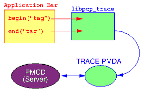
The relationship between the application, the libpcp_trace library, the trace agent and the rest of the PCP infrastructure is shown below: